Summary
This article walks you through building a “top-tier-journal–ready” correlation heatmap with hierarchical clustering in Python to analyze complex relationships between two groups of variables (e.g., microbes vs. environmental factors). You’ll learn to use Seaborn and SciPy to:
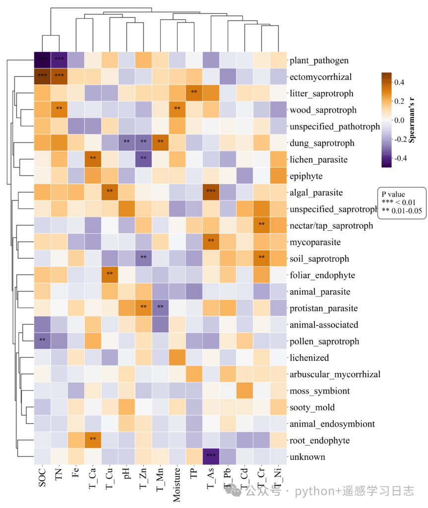
*** for p < 0.01, ** for 0.01–0.05)We’ll follow a clear workflow: read two worksheets from an Excel file (microbial data & environmental factors), align samples (rows) to keep only shared samples, compute pairwise Spearman r and p, sanitize any NaNs, render a clustered heatmap with significance markers, and export the figure.
# Core data & math
import pandas as pd
import numpy as np

# Plotting
import seaborn as sns
import matplotlib
import matplotlib.pyplot as plt

# Stats
from scipy.stats import spearmanr

# (Optional GUI backend if you run locally outside notebooks)
# matplotlib.use('TkAgg')
Why these libraries?
seaborn.clustermapWe must ensure row alignment (sample IDs) between the two tables before computing correlations.
def plot_spearman_clustermap(data1: pd.DataFrame, data2: pd.DataFrame,
                             out_path: str = "clustered_correlation.png",
                             vmax: float = 0.5):
    """
    Build a clustered heatmap of Spearman correlations between
    variables in data1 (rows) and variables in data2 (cols),
    with significance stars from p-values.

    Parameters
    ----------
    data1 : DataFrame
        Samples x variables (e.g., microbes)
    data2 : DataFrame
        Samples x variables (e.g., environmental factors)
    out_path : str
        Where to save the figure
    vmax : float
        Color scale half-range; heatmap uses [-vmax, +vmax]
    """

    # --- 1) Align on row index (sample IDs) ---
    print("\n--- Aligning sample rows between the two datasets ---")
    print(f"Before align, data1 first 5 index: {data1.index[:5].tolist()} ...")
    print(f"Before align, data2 first 5 index: {data2.index[:5].tolist()} ...")

    data1, data2 = data1.align(data2, join='inner', axis=0)
    print(f"After align, shared samples: {data1.shape[0]}")
    if data1.shape[0] == 0:
        raise ValueError(
            "Error: The two datasets have no shared sample indices. "
            "Check that sample IDs match across sheets."
        )

    # Names for heatmap axes
    rows = data1.columns  # will be heatmap rows
    cols = data2.columns  # will be heatmap cols

    # Initialize containers for r and p
    corr_matrix = pd.DataFrame(index=rows, columns=cols, dtype=float)
    p_matrix = pd.DataFrame(index=rows, columns=cols, dtype=float)
What this does
align(..., join='inner', axis=0) keeps only shared samples (row indices) so every pairwise correlation uses the same samples.Tip: For the alignment to work, both DataFrames must have sample IDs as their index. See the “Main script” section below for recommended reading options.
We compute Spearman r and p-values for every pair (each column in data1 vs. each column in data2). We also sanitize any residual NaNs.
    # --- 2) Compute Spearman r and p for each pair ---
    for r in rows:
        for c in cols:
            corr, p_val = spearmanr(data1[r], data2[c], nan_policy='omit')
            corr_matrix.loc[r, c] = corr
            p_matrix.loc[r, c] = p_val

    # Final cleanup: if any correlations are NaN (e.g., <2 valid points), set to 0
    corr_matrix.fillna(0, inplace=True)
Why Spearman?
Spearman uses ranks, making it robust to outliers and nonlinearity (monotonic but not necessarily linear relationships).
About NaNs
Even with nan_policy='omit', if too few valid data points remain, spearmanr can return NaN. We convert those to 0 so plotting won’t crash.
We convert the p-value matrix into a star annotation matrix and feed both into seaborn.clustermap. We also tune figure size, fonts, dendrogram lines, and a custom legend for p-value stars.
    # --- 3) Build significance star annotations ---
    annot_matrix = p_matrix.map(lambda p: '***' if p < 0.01 else ('**' if p < 0.05 else ''))

    # Global font tweaks
    plt.rcParams['font.sans-serif'] = ['Times New Roman']
    plt.rcParams['axes.unicode_minus'] = False

    # Dynamic size based on matrix shape
    n_rows, n_cols = corr_matrix.shape
    fig_width = n_cols * 0.5 + 4
    fig_height = n_rows * 0.5 + 4

    cmap = 'PuOr_r'   # divergent palette (purple–orange, reversed)

    # --- 4) Draw clustered heatmap ---
    g = sns.clustermap(
        corr_matrix,
        method='average',          # UPGMA
        metric='euclidean',
        cmap=cmap,
        vmin=-vmax, vmax=vmax,     # symmetric color scale
        annot=annot_matrix,
        fmt='s',                   # annotations are strings (stars)
        annot_kws={"size": 16, "color": "black", "fontweight": "bold"},
        linewidths=.5, linecolor='white',
        dendrogram_ratio=0.1,
        figsize=(fig_width, fig_height),
        cbar_pos=(1.15, 0.65, 0.03, 0.2),
        cbar_kws={'label': "Spearman's r"},
    )

    # Ticks & labels
    plt.setp(g.ax_heatmap.get_xticklabels(), rotation=90, fontsize=12)
    plt.setp(g.ax_heatmap.get_yticklabels(), rotation=0, fontsize=12)

    # Colorbar label & ticks
    g.cax.set_ylabel("Spearman's r", fontsize=12, fontweight='bold')
    g.cax.tick_params(labelsize=10)

    # Make dendrogram lines slightly thicker for clarity
    if g.ax_row_dendrogram.collections:
        g.ax_row_dendrogram.collections[0].set_linewidth(1.5)
    if g.ax_col_dendrogram.collections:
        g.ax_col_dendrogram.collections[0].set_linewidth(1.5)

    # --- 5) Manual legend for P-value stars ---
    legend_text = "P value\n*** < 0.01\n**  0.01–0.05"
    plt.text(1.15, 0.6, legend_text, transform=g.fig.transFigure,
             fontsize=11, va='top',
             bbox=dict(boxstyle='round,pad=0.5', fc='white', ec='black', lw=1))

    # Save & show
    plt.savefig(out_path, bbox_inches='tight', dpi=300, pad_inches=0.2)
    plt.show()

    return g
What you get
This is the only part you need to edit to run on your own data. It reads two sheets, sets the correct indices (sample IDs), and calls the plotting function.
if __name__ == "__main__":
# >>> EDIT THESE THREE LINES FOR YOUR DATA <<<
input_excel_path = r"your\full\path\your_data.xlsx"
sheet_name_1 = "Microbial_Guilds" # microbes (rows = samples, cols = taxa/guilds)
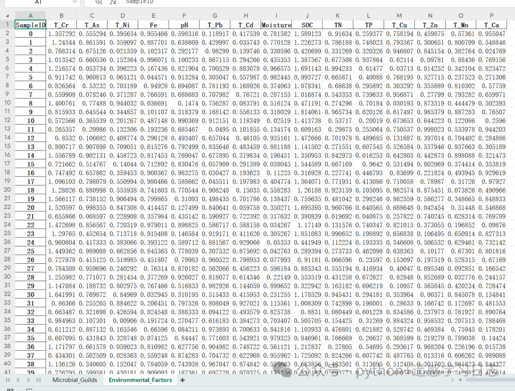
sheet_name_2 = "Environmental_Factors" # environment (rows = samples, cols = factors)
print(f"Loading data from '{input_excel_path}' ...")
# Recommended: set the **same** sample ID column as index for BOTH sheets.
# Example: if the first column in each sheet is 'SampleID', do:
microbe_data = pd.read_excel(input_excel_path, sheet_name=sheet_name_1, index_col=0)
env_data = pd.read_excel(input_excel_path, sheet_name=sheet_name_2, index_col=0)
print("Data loaded. Shapes:", microbe_data.shape, env_data.shape)
# Run the plotter (change output path if you like)
plot_spearman_clustermap(microbe_data, env_data,
out_path="clustered_correlation.png",
vmax=0.5)
Why set index_col=0 for both?
It ensures the first column (sample IDs) becomes the row index for both tables, which makes align(..., axis=0) work exactly as intended. If your IDs are in a different column, pass that column index or name to index_col.
Microbial_Guilds): rows = samples; columns = taxa/guilds; first column = SampleIDEnvironmental_Factors): rows = samples; columns = environmental variables; first column = SampleIDinput_excel_path = r'...\your_data.xlsx'sheet_name_1, sheet_name_2 to your sheet namesindex_col accordingly.clustered_correlation.png by default)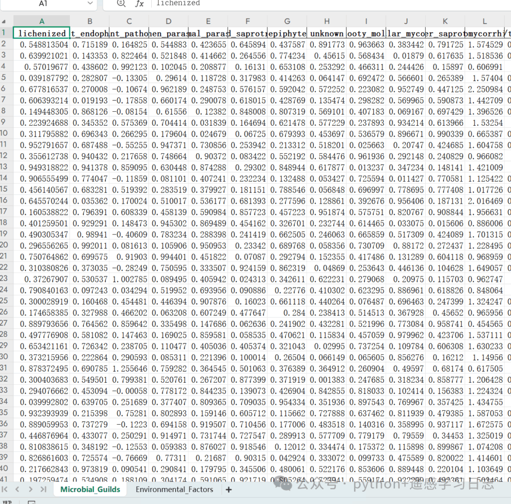
*** for p < 0.01, ** for 0.01–0.05; blank means not significant at these thresholds.statsmodels.stats.multitest.multipletests) and replace stars accordingly.vmax to emphasize stronger correlations (e.g., vmax=0.7).